HAL-PC Magazine

This column will cover features, some new some old, often overlooked by computer users, both new and long time users. We’re hoping you will incorporate at least one of the tips. We’d love to hear from you about what you find helpful. If you have any suggestions about what you would like to see covered, please email Mel Babb at melbabb@earthlink.net. Please, include your phone number so she can call you about it.

Using the Excel spreadsheet can make tasks that require doing math a snap. Most of what I’ll cover is in all newer versions of Excel. Let’s start with reconciling your checkbook to your bank statement using Excel. That way you get something useful done and learn how to use the spreadsheet, if you are new at it, and maybe learn some tricks if you already know how to use Excel. With a calculator if you make a mistake, you have to re-ad the numbers or go through gyrations that I never did master very well. With Excel, you use a formula for the total, change the number that’s wrong and voilá the total is automatically refigured.

First let’s get oriented to the spreadsheet, called a worksheet in Excel. The worksheet consists of columns which are labeled with letters and rows which are labeled with numbers. The intersection of a row and column is called a cell and has an address of a letter and column, A1, H34. When you click anywhere on the sheet the address shows in the name box in the upper left corner D2 To the right of that, the contents of the cell are displayed in the formula bar. If the contents are a formula (like =+A3+B5-C10) or a function (which is a special kind of formula, like =SUM(B3:B8)) that shows in the formula bar, otherwise the actual number or text of the cell shows. Whatever cell you click on becomes the active cell and its border becomes bold.

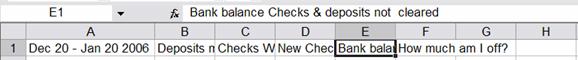
Now let’s start to create a worksheet to reconcile your checkbook to your bank statement. This is meant to show you how to use many simple handy features of Excel and is not the only or even the best way to reconcile your checkbook to your bank statement. To Start let’s type some headings in cells across row 1. In A1 type Dec 20 - Jan 20 2006 Press Enter. The cursor moves to cell A2. Since you are entering data across the row (not down the column) let’s set the cursor to move right instead of down when enter is pressed. . Click Tools, Options. Click the Edit tab. For Direction, choose Right. Click in cell B1. Ignore what’s there and just type Deposits Made. Press Enter As you start typing part of the contents of the previous cells seems to disappear. One way to fix this is to Point between the column heading A & B until a two-headed black arrow appears and double-click. The width of the cell automatically adjusts to the width needed to show all the contents in A. Finish typing the headings. Don’t adjust the column widths as you go, because an easier way will be shown later. Watch the formula bar to see what is being typed. Type: Checks Written,
New Checkbook Balance A3+ Deposits made minus Checks written,
Bank Balance Checks and Deposits not cleared,
How much am I off?
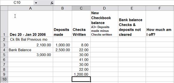
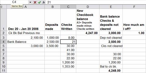
The results will look like this:

Now for some of the quick and easy ways to format this. Select (drag across the letters) columns A-F. The letters turn Black and the columns turn gray.
Right Click in the gray area, choose Format Cells.
Click the Alignment tab and check Wrap Text. OK
Right Click again, choose Column Width
Type in the number 13

Click the comma style icon, which will display the
number with a comma and 2 decimal places, (1,000.50).
Since D1 is so wordy, use a smaller font size on part of it.
Double click D1, Click after balance. Press Alt+Enter.
Select A3…written and click the drop down arrow next to the Font size icon and choose 8.
Select Row 1 by clicking on the 1.
Right Click, Format cells. Click Number tab. Click General. Now the heading line is text and not a number format which allows the font size change to display in D1.
Point to the border between row 1 and 2 until a two-headed black arrow appears and double-click. This will close up extra space in the row.
Now point to the border between A and B until a two-headed black arrow appears, Drag until all of the date shows in one line. Dragging when you see the two-headed arrow lets you decide how far you want to go. Double-clicking lets the computer decide how wide the column needs to be to display the contents of the cells. Finally, Click on row 1 and Click the bold B icon on the toolbar.
Now is a good time to save your spreadsheet. Click the save icon, and a file box appears. The File name area blank is selected with Book1.xls selected. Type in a name which will replace what is selected. (Don’t click first. If you do you’ll have to delete the Book1.xls before you can type in the name you want). Notice what folder is in the Save in blank at the top of the box. It is probably My Documents. That’s the folder the file will save in. (Change this if you wish). Click Save.
Since all the other entries are made in columns, change the cursor action back to moving down when enter is pressed. Click Tools, Options. Click the Edit tab. For Direction, choose Down. Click in cell A2 and type Ck Bk Bal Previous mo. Press enter and cursor moves to A3. Type the current check book balance 2100.
For what ever reason, I don’t calculate my balance by hand in my hand written check register. I let the computer do the math. When it’s time to reconcile, I list the previous check book balance and the new bank statement balance in column A, all the checks written since the last reconciliation in column B, and all the deposits made in column C. Fill in the columns like the example here. You do not need to type the comma or the decimal and 00. Start in cell B3.When done, click the save icon:

Use the number pad
Before putting some formulas in to make Excel do the calculating, here’s some tips. Use the number pad. If you have a desktop, the keyboard has a number key pad on the right side. If you have a laptop, you can make part of the keyboard switch to the number pad layout. Each brand of laptop may be a bit different. On my Toshiba I press and hold the blue Fn key and press the F11 key at the top of the keyboard, which has a tiny picture of a number pad on it. Notice on the keyboard which keys on the right side have tiny blue numbers on them. Click cell D2. Press number1 (if you are using a desktop and nothing happens, press the num lock key and press 1 again). Once 1 has appeared, press enter.
Start a formula with plus +

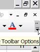A tip to keep you from having to move your hand from the number pad is to start a formula by pressing the + sign on the number pad. Just about everybody else says press the = sign, which also works but is more work! To see all the tools on the toolbars, click on the drop down arrow on toolbar options at the end of the toolbar and choose “Show Buttons on Two Rows”.

To add up Deposits made, click at the end of the deposit list, cell B5. On the tool bar click the AutoSum icon. A moving wavy outline appears around the list. Click AutoSum again. (Or Press Alt+=, then press enter). The total displays in the cell, while the function appears in the formula bar. To add up the Checks written, click at the end of the checks written list, cell C10and click twice on the AutoSum icon. Click Save

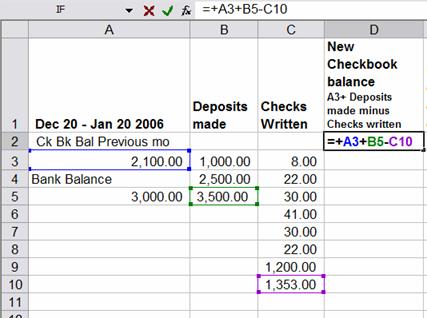
The nice thing about building formulas is that you simply click on the cell with the number you want in it, rather than typing in the cell name (A3). To calculate the new check book balance, click on D2. Press +, click A3, press +, click B5, press -, click C10, press enter. Double Click back on D2 and notice that each cell in the formula is outlined in a different color and =+A3+B5-C10 displays in the formula bar. This makes it easy to see what numbers make up the calculation. Press Esc (at the upper left on the keyboard) so no changes are made. Click Save
The Reconciliation
To do the reconciliation, click in cell E2. Press + and click on A5 to enter the bank statement balance. Press enter. To enter any deposits not cleared click E4, press + and click the cell with the uncleared deposit in it B4 Enter. That way, if you find you made a mistake typing in the deposit number, when you correct it, it will automatically correct here. Next list any unrecorded checks. Since the last 3 checks are the ones that didn’t clear yet, I’m going to enter a formula to reference the first check and then use the auto fill handle to copy the formula down and reference the other outstanding checks.

Click on E7 Type + Click C7 Enter. Click on E7, point to the lower right corner of the cell (where you see a tiny black square called the fill handle). A two-headed black arrow appears. Click and drag the handle down two cells. The formulas are copied. (Look in the formula bar to see the formula or double click the cell. If you double click remember to press Esc so no changes are made.) By the way, if you see a moving dashed outline around a cell or cells, press Esc to make it disappear. (I call this the moving ants. Microsoft calls it a moving border or animated border). It indicates what you selected. 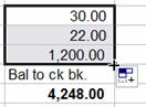(Note if you have turned on the Fn keypad on a laptop you have to toggle it off before you can type text again). Then type in E10, Bal to ck bk. In the next cell down create this formula +E2+E4-E7-E8-E9 and press enter. If you add an extra + before pressing enter an error message shows. Click Yes and the extra + will be removed for “operator” means a +,-,*, or / (an add, subtract, multiply, or divide) math sign and “operand” means the cell reference A3. The little square symbol is a smart tag. These things appear to give you options to what you just did. When you start doing something else, they will disappear.
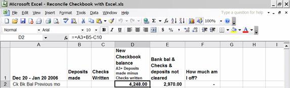
In this example, we are one dollar out of balance. Many times the amount is not that easy to figure, so let Excel do it by creating a formula that takes the checkbook balance and subtracts the bank balance from it to see the difference. Then it’s a matter of looking for that difference and correcting it, (otherwise known as the hair pulling out time). In this case, when the checks written were compared again to what cleared the bank, The 22.00 entry should have been 21. When 21 is entered in cell C4, the account is reconciled. And one last time Click Save. I think you get the message, save and save often!

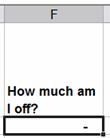
The – (dash) indicates no difference exists.
In describing this procedure, I have explained many of the symbols you encounter doing the steps in hopes that you will now recognize they are helpful not baffling.
Till next time. Happy Computing.
Mel Babb © 2006
Mel Babb, a long time member of Hal-PC, is currently an instructor and on the volunteer help committee at Hal-PC. She runs her own company, PC Tutoring Services. She comes to your home and creates notes for you on what you want to learn. Contact her at 713-981-5641 or email at melbabb@earthlink.net.

Tips and Tricks for Using Software Effectively by Mel Babb

Tips and Tricks for Using Software Effectively
by Mel Babb