Excel Formula Sense
Mel Babb
Let’s go over the basics of using formulas in Excel so you can get Excel to do more of the calculating work. After all, that’s one of the things Excel was designed to do excellently. By the way, most of what’s in this article also applies to other spreadsheet programs, like Microsoft Works and Quattro Pro. Excel is a spreadsheet program consisting of a grid of columns and rows in which among other things you enter numbers. Then you enter formulas and functions (special kinds of formulas) that perform mathematical calculations on the numbers you select and or enter in a formula.
How Excel Interprets a Formula
 Understanding how Excel processes information is absolutely necessary to getting the formula to produce the answer you want. When Excel runs a complicated calculation, it follows the basic algebra order of mathematical operations. It does not process the formula from left to right like we normally read. Instead, it processes in this order: 1) anything in parentheses (); 2) does exponents, ^ (e.g., a number raised to a power of 2, 3, etc. like 52); 3) multiplies and divides */; adds and subtracts +-. Look at Figure 1 to see how this calculates: (6+9)* 2^2/3-2. Understanding how Excel processes information is absolutely necessary to getting the formula to produce the answer you want. When Excel runs a complicated calculation, it follows the basic algebra order of mathematical operations. It does not process the formula from left to right like we normally read. Instead, it processes in this order: 1) anything in parentheses (); 2) does exponents, ^ (e.g., a number raised to a power of 2, 3, etc. like 52); 3) multiplies and divides */; adds and subtracts +-. Look at Figure 1 to see how this calculates: (6+9)* 2^2/3-2.

So to make this perfectly clear: 3+5*2=13 and (3+5)*2=16. Following the rules, the first example multiplies first then adds, while the second example adds what is in the parentheses first, then multiplies. An exponent is indicated with the ^ caret sign between the number and the power, so 3^2 means 32, three squared. You can have more than one set of parentheses in a formula. When that happens, the inner most set of parentheses is done first.
Some Terminology
Creating formulas in Excel (or math for that matter) is rule bound. If you don’t create formulas often, the rules called syntax can seem as complex and convoluted as income tax instructions. In fact, the syntax is very logical. The information that goes into a formula or function is called an argument. The most common kind of arguments are numbers (called values), cell references (like A12, or G80), Range names (explained below) or text. The math symbols like +,-,*,/ in the formulas are called operators. A cell is described by a column letter and row number, G3, M100. A1 is the first cell in a sheet. A sheet consists of 255 columns and 65,536 rows. The first 26 columns are labeled A-Z, the next 26 AA-AZ, and so forth to IV which is column 255.
What’s the Big Deal About Formulas?

The beauty of creating formulas with cell references rather than numbers (values) is that if a number in the cell used in a formula is changed, the formula automatically recalculates with the new information. So in figure 2 the formulas in B4 and C4 contains cell references: =B2-B3 and =C2-C3. (What’s shown in B5 and D5 is just to show the formulas in B4 and D4 for this example). So when 3500 is changed to 3000 in C3, the balance in C4 is updated to 2000. However, when the formula contains numbers as is D4 (which is displayed in D5) the balance does not change. The point is that in formulas you refer to the cell that has the number in it. You do not type the number directly in the formula. Here’s the best way to enter a formula using cell references. Open up a spreadsheet and type in the information in Figure 2 except for the formulas. Note as you type the formula (described in the next few sentences) the visual aids and colors that appear to help you be sure you get the right cells. To create a formula, type an = or a + in the cell where you want the answer, in this example B4. Click on the cell that has the number you want, B2. Press the – (minus) sign. Click on B3. Press Enter. When you click a cell, moving dotted lines (called a marquee) appear on that cell to let you know you have selected it. The answer cell now shows the cell reference B2 in blue. When you type the – (minus) sign, the cursor is back in the cell where you want the answer and the B2 cell is outlined in blue. When you click the next cell you want, B3, it shows the marquee and the answer cell now shows the cell reference B3 in green. Press enter to finish the formula. The cursor moves to the next cell and the result shows in the answer cell. To edit the formula or see what cells are referenced in it, double click the answer cell. The cell references B2, B3, show up in color and the actual cells are outlined in the same color, making it easy to see if you have the cells you want for your formula. This is the point and click method of entering a formula. Of course, you can always type each reference directly in the answer cell, (which used to be the only way); the cell referenced will display a colored outline.
Try These You’ll Like Them
Entering a formula is easier than describing it. Note that a formula can have a mixture of cell references and real numbers. Using the same example from figure 2, type in B6 =B4*2, to double the balance to 3000.
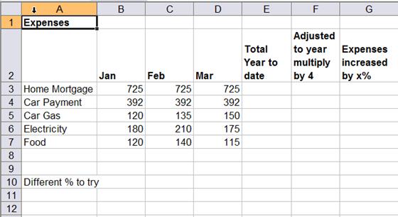
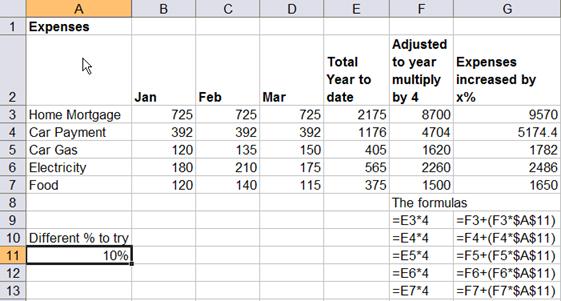
 Using a simple spreadsheet of expenses, let’s use the Sum function to total expenses and then see what happens if we increase expenses by 5, 10 or 15%. Once the raw numbers are in, and one formula is created, in this case a SUM function, that function can be copied to total the other expenses. Type the information in figure 3 into a spreadsheet. Click in cell B8. That’s where you want the total for Jan expenses. Click the AutoSum icon on the standard toolbar. Since adding up figures is one of the most common things done in spreadsheets, an icon exists to make that easy. Notice that a marquee appears around the numbers to be totaled. Click the icon again or just press enter and the column is totaled. To copy the formula to C8 and D8, use the Fill handle Using a simple spreadsheet of expenses, let’s use the Sum function to total expenses and then see what happens if we increase expenses by 5, 10 or 15%. Once the raw numbers are in, and one formula is created, in this case a SUM function, that function can be copied to total the other expenses. Type the information in figure 3 into a spreadsheet. Click in cell B8. That’s where you want the total for Jan expenses. Click the AutoSum icon on the standard toolbar. Since adding up figures is one of the most common things done in spreadsheets, an icon exists to make that easy. Notice that a marquee appears around the numbers to be totaled. Click the icon again or just press enter and the column is totaled. To copy the formula to C8 and D8, use the Fill handle  point at the fill handle in the lower right corner of B8 until a black cross appears. Drag over cells C8 and D8. The formula is copied. Feb and Mar are now totaled. Click in E3, the total for year to date. Click the AutoSum icon, note the marquee, press enter. Copy the formula down using the fill handle. point at the fill handle in the lower right corner of B8 until a black cross appears. Drag over cells C8 and D8. The formula is copied. Feb and Mar are now totaled. Click in E3, the total for year to date. Click the AutoSum icon, note the marquee, press enter. Copy the formula down using the fill handle.
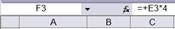
Create a formula in F3 to project the expenses for a year. Type =, click E3, type*, type 4, press enter. Move the cursor to F3 The formula =E3*4 appears in the formula bar at the top of the screen and the answer in the cell.
There’s one more thing to cover about basic formula creation: the difference between relative and absolute cell reference. Sometimes when you copy a formula from one place to another, you want part of the formula to keep referring to exactly (absolutely) the same cell. In the expenses example this happens when you want to put a percentage increase into expenses. Part of the formula needs to move down a row as it is copied (move relative to where the answer is) and part of it needs to keep referring exactly (absolutely) to the same row and column. An indicator needs to be put in the part of the formula that stays constant. That indicator is a $ (dollar sign), which is entered by pressing the F4 (function 4) key.
Try this example. In A11 type 10%, the percentage to increase expenses. In cell G3 type =, click F3, type (, click F3 again, press +, then ). Press *, Click A11, Press the function key F4, Press enter. Move the cursor back to G3. The formula bar displays =F3+(F3*$A$10). When you copy the formula down the F3 moves to F4 then F5, etc. while the A11 stays put. If you forget to press the F4 key, you can double click on G3 and click on the A11 side of the formula and press the F4 key to edit the formula. Then copy it down again. Try changing the percentage in A11 to 5% or 8% and watch the numbers in column G change. Now go ahead and see what kind of formulas you can create on your own.

Till next time. Happy Computing
Mel Babb © 2006
Mel Babb, a long time member of HAL-PC, is currently an instructor at various places in town and on the Volunteer Help committee at HAL-PC. She runs her own company, PC Tutoring Services. She comes to your home and creates notes for you on what you want to learn. See her website www.melpchelp.com or contact her at mel@melpchelp.com .
|